
The next step in answering questions related to seasonal performance is to combine the performance information for the heat pump and house with climate data for Boston.
Because the heating capacity of an air-to-water heat pump is highly dependent on outdoor air temperature, its seasonal performance will depend on the time during which the heat pump operates at different outdoor temperatures. Data for long-term averages of hourly outdoor temperature is readily available for hundreds of locations in North America. Sources for this data include:
• ACCA manual J
• ASHRAE Weather Data Viewer software
Figure 5-4 shows an example of “bin” temperature data for Boston, MA. In this case, the “bins” are 5ºF wide. Each vertical bar gives the number of hours that the outdoor temperature falls within the specified range, based on long-term average values for those temperatures. On any specific year, the number of hours in each bin may be higher or lower than the long-term average.
The outdoor design temperature in Boston is 9ºF. Notice how many hours correspond to outdoor temperatures significantly higher than this design temperature. This implies that most of the heating occurs under partial load conditions.
If internal heat gains are minimal, and thermostat setbacks are not used, space heating loads can be modeled as being approximately proportional to the difference between the indoor setpoint temperature and the outdoor temperature. This allows the heating load to be calculated as a percentage of design heating load using the average outdoor temperature for each bin. Figure 5-5 shows a spreadsheet where this has been done, based on the Boston bin temperature data shown in Figure 5-4.


The right side column in Figure 5-5 gives the hours during which the space heating load equals or exceeds each given percentage of design load. Plotting the last two columns of this spreadsheet up to outdoor temperatures of 65ºF yields a “heating duration curve,” as shown in Figure 5-6.

The yellow shaded area under the heating duration curve is approximately proportional to the total space heating energy needed over an average heating season. This is based on the assumption that internal heat gains alone supply the home’s heat loss at outdoor temperatures of 65ºF or higher.
The relationship between the area under the heating duration curve and the total seasonal space heating energy required can be very useful when combined with other building and heat pump performance data. Figure 5-7 shows one example.
The graph of heat pump heating capacity and building supply water temperature (on right) is shown next to the heating duration curve for Boston. The graphs have been scaled so that the design heating load of 75,000 Btu/hr on the right graph aligns with the 100% of design load on the left graph. A line has been drawn horizontally from the balance point on the right graph to the vertical axis of the other graph. The green shaded area under this line represents about 94% of the total area under the heating duration curve. This implies that, on an average year, the selected heat pump alone supplies about 94% of the total space heating energy while operating at or above the outdoor balance point temperature. The remaining space heating energy is supplied through the combined operation of the heat pump and a supplemental heat source.
The same horizontal line can be extended to the supply water temperature scale on the right graph. This shows that for 94% of the heating season, the required supply water temperature is at or below 103ºF, a temperature that allows modern air-to-water heat pumps to run at relatively high COP.
The low-ambient air-to-water heat pump assumed in this example could operate down to an outdoor temperature of -5ºF. On an average year in Boston, there is only 1 hour of outdoor temperature lower than -5ºF. Thus, the heat pump would remain in operation over essentially the full range of outdoor air temperature. The required supply water temperature corresponding to an outdoor temperature of -5ºF would be about 132ºF. The low- ambient heat pump used in this example would have a COP of about 1.7 under this condition.

SPREADSHEET MODELING OF SYSTEM PERFORMANCE
Previous discussions have shown the variability of heating capacity and COP based on changes in the temperature of water leaving the heat pump’s condenser and the outside air temperature.
The building that the heat pump serves also experiences wide changes in heating load over the heating season.
Hydronic distribution systems that use outdoor reset control to avoid “overheating” the water supplied to the distribution system will minimize the required supply water temperature, and thus, enhance the heat pump’s performance under partial load conditions. These systems will experience a wide range of supply water temperatures.
The geographic location where the heat pump is installed will have specific average values for each temperature bin.
All these variables make it impossible to provide an accurate “rule of thumb” for sizing an air-to-water heat pump on a given project.
The preferred approach is to simulate a proposed system configuration by building a spreadsheet that includes reasonable mathematical models for the building load, performance of the heating distribution system, performance of the heat pump and outdoor air temperature for the location of the project. Once the simulation spreadsheet is built, the designer can experiment with various “what if” scenarios on equipment size, supply water temperatures, etc., to determine overall seasonal performance and make decisions on system design.
The following mathematical models were used to build a simulation spreadsheet that merges the thermal performance of the previous discussed building, a nominal 4-ton low-ambient air-to-water heat pump, the building’s heating distribution system and climatic data for Boston. These calculations were performed for each bin of outdoor temperature. The outdoor temperature (Tamb) is taken as the average temperature of each bin (i.e., for the 15–20ºF bin, Tamb would by 17.5ºF).

Instantaneous building space heating load:
$${L_{bldg}} = {{Q_{d}} \over{ΔT_{d}}} · {({T_{i})-({T_{out})}}}-{Q_{i}} $$
Where:
Lbldg = instantaneous building space heating load (Btu/hr)
Qd = building’s design space heating load (Btu/hr)
ΔTd = difference between inside and outside temperature at design load (ºF)
Tin = indoor setpoint temperature for space heating (ºF),typically assumed at 70ºF
Tout = current outdoor temperature (ºF)
Qi = current rate of internal heat gain (Btu/hr)
Supply water temperature to space heating distribution:
$${T_{s}} = {{{{T_{sd}}-{T_{in}}}}\over{{{T_{in}}-{T_{od}}}}} · {({T_{in}-{T_{out})}}}+{T_{in}} $$
Where:
Ts = currently required supply water temperature (ºF)
Tsd = required supply water temperate at design load (ºF)
Tin = indoor setpoint temperature for space heating (ºF), typically assumed at 70ºF
Tod = outdoor temperature at design load (ºF)
Toutb = current outdoor temperature (ºF)

Heating capacity of heat pump:
$$Q_h=[{k_1+k_2(T_s)]+k_3(T_{out})+k_4(T_{out})^2} $$
Where:
Qh = “instantaneous” heating capacity of heat pump (Btu/hr)
Ts = currently required supply water temperature to distribution system (ºF)
Tout = current outdoor temperature (ºF)
k1, k2, k3, k4 = constants determined by curve fitting tomanufacturer’s published heat capacity curves.
COP of heat pump:
$$COP=[{c_1+c_2(T_s)+c_3(T_{amb})+c_4(T_{amb})^2} $$
Where:
COP = “instantaneous” COP of heat pump (Btu/hr)
Ts = currently required supply water temperature to distribution system (ºF)
Tamb = current outdoor temperature (ºF)
c1, c2, c3, c4 = constants determined by curve fitting to manufacturer’s published heat capacity

The modeling equations for the heat pump’s heating capacity and COP are based on curve fitting, which provides an approximation of performance over a range of operating conditions. These modeling equations may not accommodate the performance characteristics of all air-to-water heat pumps, or the characteristics of all building loads or heating distribution systems. In some cases, designers may need to use other modeling methods to achieve accurate simulation.

Any models developed should be checked to see if they can replicate published performance information with reasonable accuracy. It’s also important to remember that curve fitting is based on specific ranges of data. The equations developed from curve fitting should only be applied within those ranges of data unless specific constraints are imposed, such as limiting maximum heating capacity and COP values under very desirable operating conditions. Check with heat pump manufacturers to verify such constraints
SEASONAL AVERAGE COP
It is possible to use performance information for the heat pump and the building’s hydronic heating distribution system, combined with bin temperature data for a given location, to calculate a “project-adjusted” seasonal average COP. This involves determining the required supply water temperature for each bin, using this temperature along with the corresponding outdoor temperature and the heat pump’s COP data (or model) to determine the COP for that bin. The operating hours of the heat pump in each bin are calculated. These values cannot exceed the actual hours in each bin. The operating hours in each bin are multiplied by the COP for that bin. These multiplications are summed and then divided by the total heat pump operating hours over the heating season to get a project-adjusted average COP for the heating season. These calculations are best done using a spreadsheet.
When this method was applied to the previously discussed building near Boston, along with the constraint that the maximum COP could not exceed 4.5, and the heating capacity could not exceed 72,000 Btu/hr, the seasonal average COP of the heat pump was 3.49. This is an excellent performance number that is comparable to, if not higher than, what the seasonal average COP of a geothermal heat pump of the same capacity, and applied under the same conditions, might be. This seasonal average COP is based on the full outdoor temperature range for an average Boston winter, which ranges from -10ºF to a high of 70ºF.
Additional spreadsheet-based analysis of this example project indicates that the total space heating energy required for the building for an average Boston winter is 194.3 MMBtu ( 1 MMBtu = 1,000,000 Btu). Of this, the heat pump supplied 185.0 MMBtu (about 95% of total), and the auxiliary heat source supplied 9.3 MMBtu (about 5%) of total.
As of this writing, the cost of electricity supplied to residential customers just west of Boston, where the building is located, is \$0.149/kwhr. This is slightly higher than the current U.S. national average rate of \$0.118/kwhr. If electricity costing \$0.149/kwhr was directly converted to heat, such as in an electric boiler, the cost per million Btus would be \$43.66/MMBtu. This would make the estimated seasonal heating cost of the building $8,483.
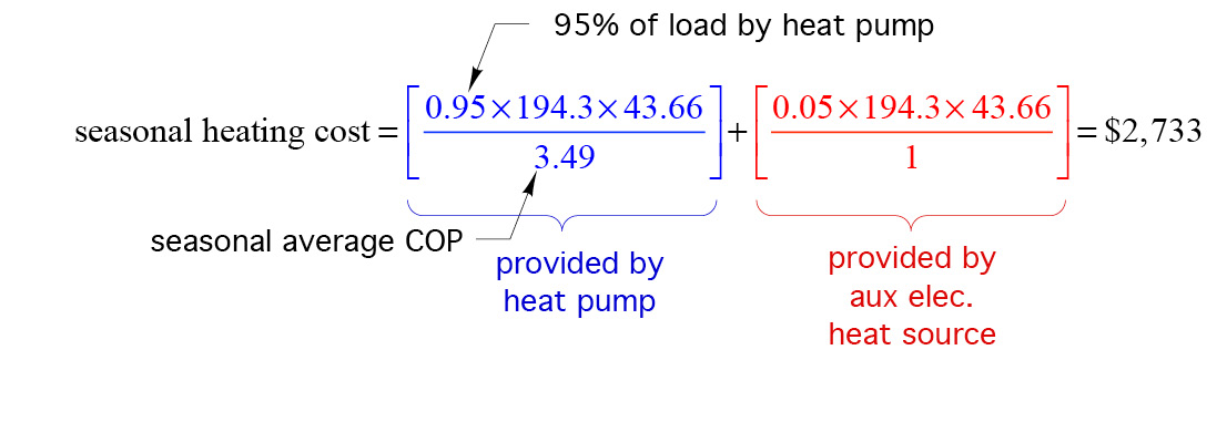
Assuming that the air-to-water heat pump, operating at a seasonal average COP of 3.49, supplies 95% of the seasonal heat — both of which were projected by the spreadsheet analysis — and that an electric boiler supplies the remaining 5%, the estimated seasonal heat cost would be:
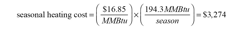
The current price of natural gas in Boston is about \$1.55 per therm, which at an assumed 92% seasonal average boiler efficiency equates to \$16.85/MMBtu. The cost of heating the example house for an average winter using natural gas at this rate and conversion efficiency would be:
In this project, the cost of space heating energy using the air-to-water heat pump was 16.5% lower than using natural gas. Furthermore, if a basic service charge of \$20 per month for having a natural gas meter on the building was eliminated so that the house was all electric, an additional savings of \$240 per year would be achieved. The total annual savings would be $781 per year. This example has shown that the majority (95%) of the space heating energy for a house near Boston with a 75,000 Btu/hr design load, and a hydronic distribution system that requires 120ºF water at design conditions, can be supplied by a nominal 4-ton low-ambient air-to-water heat pump, and at seasonal cost about 16% lower than if the heating was done using a high-efficiency boiler operating on natural gas.