
PREFACE

Water is the essential ingredient in any hydronic system. Its physical properties make it possible to deliver heating or cooling throughout a building using relatively small “conduits” and minimal amounts of electrical energy.
The performance of all hydronic systems is intimately tied to the physical properties of water—in particular, the process by which water absorbs heat, conveys it and releases it. This section discusses the fundamental relationships that govern those processes. It discusses properties that affect both the thermal and hydraulic performance of all hydronic systems. It clarifies the differences as well as the interrelationships between physical quantities such as temperature, heat content, rate of heat transfer, flow rate, flow velocity, head energy and pressure drop.
Understanding these physical properties and how they are related is essential for anyone who wants to design efficient and reliable hydronic systems. Such an understanding is also important for those who diagnose and adjust hydronic systems for optimal performance.
SENSIBLE HEAT & LATENT HEAT
The heat absorbed or released by a material while it remains in a single phase is called sensible heat. The word sensible means that the presence of the heat can be sensed by a temperature change in the material. When a material absorbs sensible heat, its temperature must increase. Likewise, when a material releases sensible heat, its temperature must decrease. Under normal operating conditions, all the hydronic systems discussed in this and other issues of idronics operate with water that remains in liquid form. Thus, all heat and heat transfer quantities discussed are sensible heat.
If a material changes phase while absorbing heat, its temperature does not change. The heat absorbed in such a process is called latent heat. For water to change from a liquid to a vapor, it must absorb approximately 970 Btu/lb. This is a very large amount of heat to be conveyed by a single pound of material. It is also the physical characteristic that is leveraged by a steam heating system.
SPECIFIC HEAT & HEAT CAPACITY


By comparing the heat capacity of water and air, it can be shown that a given volume of water can hold almost 3,500 times as much heat as the same volume of air for the same temperature rise. This allows a given volume of water to transport vastly more heat than the same volume of air. This is the underlying (and very significant) advantage of using water rather than air for moving sensible heat. Figure 5-3 illustrates this advantage by comparing two heat transport systems of equal heat-carrying ability. The 1” diameter tube carrying water can convey the same amount of heat as a 10” by 20” duct conveying air when both systems are operating at typical temperature differentials and flow rates.
DENSITY

In this and other issues of idronics, the word “density” refers to the number of pounds of the material needed to fill a volume of one cubic foot. For example, it would take 62.4 pounds of water at 50ºF to fill a 1 cubic foot container, so its density is said to be 62.4 pounds per cubic foot, (abbreviated as 62.4 lb/ft^3 ).
The density of water varies with its temperature. Like most substances, as the temperature of water increases, its density decreases. As temperature increases, each molecule of water requires more space. This molecular expansion is extremely powerful and can easily burst metal pipes or tanks if not properly accommodated. Figure 5-4 shows the relationship between temperature and the density of water.
The change in density of water or water-based antifreeze solutions directly affects the size of the expansion tank required on all closed-loop hydronic systems. Proper tank sizing requires data on the density of the system fluid both when the system is filled and when it reaches its maximum operating temperature.
The change in water’s density based on its temperature affects several other aspects of hydronic system design and operation. For example, because hot water is less dense than cool water, it will rise to the top of a thermal storage tank. The difference in density between warm and cool water in different parts of the system was also responsible for creating circulation in early hydronic systems, as discussed in section 3.
SENSIBLE HEAT QUANTITY FORMULA
It is often necessary to determine the quantity of heat stored in a given volume of water that undergoes a temperature change. Formula 5-1, known as the sensible heat quantity formula, can be used for this purpose:
$$ h = 8.33v \bigl( \Delta T \bigr) $$
Where:
$h$ = quantity of heat absorbed or released from the water
(Btu) $v$ = volume of water (gallons)
$\Delta T$ = temperature change of the material (ºF)
Example: Assume a storage tank contains 500 gallons of water initially at 70ºF. How much heat must be added to raise this water to a temperature of 180ºF?
Solution: The amount of heat involved is easily determined using Formula 5-1:
$$ h = 8.33v \bigl( \Delta T \bigr) = 8.33 \times 500 \times (180-70) = \text{458,000} \ Btu $$
SENSIBLE HEAT RATE FORMULA
Hydronic system designers often need to know the rate of heat transfer to or from a fluid flowing through a device such as a heat source or heat emitter. This can be done using the sensible heat rate formula, given as Formula 5-2:
$$ h = (8.01Dc) f( \Delta T) $$
where:
$Q$= rate of heat transfer into or out of the water stream (Btu/hr)
$8.01$= a constant based on the units used
$D$= density of the fluid (lb/ft^3 )
$c$= specific heat of the fluid (Btu/lb/ºF)
$f$= flow rate of fluid through the device (gpm)
$\Delta T$= temperature change of the fluid through the device (ºF)
When using Formula 5.2, the density and specific heat should be based on the average temperature of the fluid during the process by which the fluid is gaining or losing heat.

For cold water only, Formula 5-2 simplifies to Formula 5-3:
$$ q = 500f (\Delta T) $$
where:
$Q$= rate of heat transfer into or out of the water stream (Btu/hr)
$f$= flow rate of water through the device (gpm)
$500$= constant rounded off from 8.33 x 60
$\Delta T$= temperature change of the water through the device (ºF)
Formula 5-3 is technically only valid for cold water because the factor 500 is based on the density of water at approximately 60ºF. However, because the factor 500 is easy to remember, Formula 5-3 is often used for quick mental calculations for the rate of sensible heat transfer involving water. While this is fine for initial estimates, it is better to use Formula 5-2 for final calculations because it accounts for variations in both the density and specific heat of the fluid. Formula 5-2 can also be used for fluids other than water.
Example: Water flows into a radiant panel circuit at 110ºF and leaves at 92ºF. The flow rate is 1.5 gpm, as shown in Figure 5-5. Calculate the rate of heat transfer from the water to the heat emitter using:
a. Formula 5-2
b. Formula 5-3
Solution: Using Formula 5-2, the rate of heat transfer from the circuit is:
$$ q = 500f( \Delta T) = 500 \times 1.5 \times (110-92) = \text{13,500} \ Btu/hr$$
To use Formula 5-3, the density of water at its average temperature of 101ºF must first be estimated using Figure 5-4:
$$ D = 61.96 \ \text{lb/ft}^3 $$
The specific heat of water can be assumed to remain 1.0 Btu/lb/ºF
Putting these numbers into Formula 5-2 yields:
$$ q = (8.01Dc) f( \Delta T) = (8.01 \times 61.96 \times 1.00) \times1.5 \times (110-92) = \text{13,400} \ Btu/hr $$
The difference in the calculated rate of heat transfer is small, only about 0.7%. However, this difference will increase as the water temperature in the circuit increases.
Formula 5-2 is generally accepted in the hydronics industry for quick estimates of heat transfer to or from a stream of water. However, Formula 5-3 yields slightly more accurate results when the variation in density and specific heat of the fluid can be factored into the calculation.
Formulas 5-2 and 5-3 can also be rearranged to determine the temperature drop or flow rate required for a specific rate of heat transfer.
Example: what is the temperature drop required to deliver heat at a rate of 50,000 Btu/hr using a distribution system operating with water at a flow rate of 4 gpm?
Solution: Just rearrange Formula 5-2 and put in the numbers.
$$ \Delta T = {q \over 500f} = {\text{50,000} \over 500 \times 4} = 25^o F$$
Example: What is the flow rate required to deliver 100,000 Btu/hr in a distribution system that operates with water and a temperature drop of 30ºF?
Solution: Again, Formula 5-2 can be rearranged to determine flow and the known values factored in.
$$ f = {q \over 500 (\Delta T)} = {\text{100,000} \over 500(30)} = 6.7gpm $$
Formula 5-2 and the slightly more accurate Formula 5-3 are perhaps the most important formulas in hydronic system design. They are constantly used to relate the rate of heat transfer to fluid flow rate and the temperature change of the fluid.
VAPOR PRESSURE AND BOILING POINT
The vapor pressure of a liquid is the minimum pressure that must be applied at the liquid’s surface to prevent it from boiling. If the pressure on the liquid’s surface drops below its vapor pressure, the liquid will instantly boil. If the pressure is maintained above the vapor pressure, the liquid will remain a liquid and no boiling will occur.
The vapor pressure of a liquid is depends on its temperature. The higher the liquid’s temperature, the higher its vapor pressure. Stated another way, the greater the temperature of a liquid, the more pressure must be exerted on its surface to prevent it from boiling.
Vapor pressure is stated as an absolute pressure and has the units of psia. On the absolute pressure scale, zero pressure represents a complete vacuum. On earth, the weight of the atmosphere exerts a pressure on any liquid surface open to the air. At sea level, the absolute pressure exerted by the atmosphere is approximately 14.7 psia.

Figure 5-6 shows this relationship between the vapor pressure and temperature of water between 50ºF and 250ºF.
The vapor pressure of water at 212ºF is 14.7 psia. Because 14.7 psia is the absolute pressure the atmosphere exerts at sea level, and water at sea level boils at 212ºF.
If a pot of water is carried to an elevation of 5,000 feet above sea level and then heated, its vapor pressure will rise until it equals the reduced atmospheric pressure at this elevation, and boiling will begin at about 202ºF. Conversely, if a container of water is sealed from the atmosphere and pressurized to about 15.3 psi above atmospheric pressure (e.g., to an absolute pressure of 30 psia), Figure 5-6 indicates that the water must be heated to about 250ºF before it will boil.
Closed-loop hydronic systems should be designed to ensure that the absolute pressure of the water at all points in the system remains safely above the water’s vapor pressure under all operating condition. This prevents problems such as cavitation in circulators and valves or “steam flash” in piping.
VISCOSITY
The viscosity of a fluid is an indicator of its resistance to flow. The higher the viscosity of a fluid, the more drag it creates as it flows through pipes, fittings, valves or any other component in a hydronic circuit. Higher viscosity fluids also require more pumping power to maintain a given flow rate compared to fluids with lower viscosities.
The viscosity of water depends on its temperature. The viscosity of water and water-based antifreeze solutions decreases as their temperature increases.
Solutions of water and glycol-based antifreeze have significantly higher viscosities than water alone. The greater the concentration of antifreeze, the higher the viscosity of the solution. This increase in viscosity can result in significantly lower flow rates within a hydronic system if it is not accounted for during design.
DISSOLVED AIR IN WATER
Water can absorb air much like a sponge can absorb a liquid. Molecules of the gases that make up air, including oxygen and nitrogen, can exist “in solution” with water molecules. Even when water appears perfectly clear, it often contains some dissolved air.
When hydronic systems are first filled, dissolved air is present in the water throughout the system. If allowed to remain in the system, this air can create numerous problems, including noise, cavitation, corrosion, inadequate flow or even complete flow blockage.
A well-designed hydronic system must be able to automatically capture dissolved air and expel it. A proper understanding of what affects the air content of water is crucial in designing a method to get rid of it.
The amount of air that can exist in solution with water is strongly dependent on the water’s temperature. As water is heated, its ability to hold air in solution rapidly decreases. However, the opposite is also true. As water cools, it has a propensity to absorb air. Heating water to release dissolved air is like squeezing a sponge to expel a liquid. Allowing the water to cool is like letting the sponge expand to soak up more liquid. Together these properties can be exploited to help capture and eliminate air from the system.
The water’s pressure also affects its ability to hold dissolved air. When the pressure of the water is lowered, its ability to contain dissolved air decreases, and vice versa.
Figure 5-7 shows the maximum amount of air that can be contained (dissolved) in water as a percentage of the water’s volume. The effects of both temperature and pressure on dissolved air content can be determined from this graph.
To understand this graph, first consider a single curve such as the one labeled 30 (psi). This curve represents a constant pressure condition for the water. Notice that as the water temperature increases, the curve descends.
This indicates a decrease in the ability of water to contain dissolved air as its temperature increases. This trend also holds true for all other constant pressure curves.
The vertical axis of the graph indicates the maximum possible amount of dissolved air in water. This condition represents water that is “saturated” with dissolved air, and thus unable to absorb any more air.
The water in a properly deareated hydronic system will eventually hold much less dissolved air than the numbers on the vertical axis indicate. Under this condition, the water would be described as “unsaturated.” This means it can absorb air it comes in contact with within the system. High-performance air separators, such as a Caleffi Discal, maintain system water in this unsaturated state, and thus enable it to absorb air pockets that might form within the system due to component maintenance or other reasons.
The change in the ability of water to retain air can be read by subtracting values on the vertical axis. For example, at an absolute pressure of 30 psia and temperature of 65ºF, the maximum amount of dissolved air is 3.6 gallons of air per 100 gallons of water. If that water is then heated to 170ºF and its pressure is maintained at 30 psia, its ability to hold air in solution has decreased to about 1.8 gallons of air per 100 gallons of water. Thus, the amount of air released from the water during this temperature increase is estimated at 3.6-1.8 = 1.8 gallons per 100 gallons of water.
The release of dissolved air can be observed in a kettle of water that is being heated on a stove. As the water heats up, bubbles will form at the bottom of the kettle (e.g., where the water is hottest). These bubbles are formed as gas molecules that were dissolved in the cool water are forced out of solution by increasing temperature. The molecules join together to create bubbles. This process is called coalescing. If the kettle of water is allowed to cool, these bubbles will disappear as the gas molecules go back into solution.
One can think of the dissolved air initially contained in a hydronic system as being “cooked” out of the solution as water temperature increases. This usually takes place inside the heat source when it is first operated after being filled with “fresh” water containing dissolved gases. Well-designed hydronic systems take advantage of this situation by capturing air bubbles with an air separator that is typically placed near the outlet of the heat source (e.g., where the water is hottest).
For a more in-depth discussion on Hydronic Systems:
INCOMPRESSIBILITY
STATIC PRESSURE
Static pressure develops within a fluid due to its own weight. The static pressure that is present within a liquid depends on the depth of the liquid below (or above) some reference elevation.
Consider a pipe with a cross-sectional area of 1 square inch filled with water to a height of 10 feet, as shown in Figure 5-8.
Assuming the water’s temperature is 60ºF, its density is 62.4 lb/ft3 . The weight of the water in the pipe could be calculated by multiplying its volume by its density.
$$ \text{Weight} = \left( 1 \ \text{in}^2 \right) \left( 10 \ \text{ft.} \right) \left( 62.4{\text{lb} \over \text{ft}^3} \right) \left( 1\text{ft}^2 \over 144\text{in}^2 \right) = 4.33\ \text{lb}$$
The water exerts a pressure on the bottom of the pipe due to its weight. This pressure is equal to the weight of the water column divided by the area of the pipe. In this case:
$$\text{Static pressure} = {\text{weight of water} \over \text{area of pipe}} = {4.33 \ \text{lb} \over \text{1 in}^2} = 4.33 {\text{lb} \over \text{in}^2} = 4.33 \text { psi}$$
If a very accurate pressure gauge were mounted into the bottom of the pipe, as shown in Figure 5-8, it would read exactly 4.33 psi.
The size or shape of the “container” holding the water has no effect on the static pressure at any given depth.
Thus, an accurate pressure gauge placed 10 feet below the surface of a lake containing 60ºF water would also read exactly 4.33 psi.

The size or shape of the “container” holding the water has no effect on the static pressure at any given depth.
If a very accurate pressure gauge were mounted into the bottom of the pipe, as shown in Figure 5-8, it would read exactly 4.33 psi. Thus, an accurate pressure gauge placed 10 feet below the surface of a lake containing 60ºF water would also read exactly 4.33 psi.
The static pressure of a liquid increases proportionally from some value at the surface to larger values at greater depths below the surface. Formula 5-4 can be used to determine the static pressure below the surface of a liquid.
$$ P_{static}= \left( D \over144 \right) h \ + P_{static} $$
where:
$P_{static} = $static pressure at a given depth, h, below the surface of the water (psi)
$h$ = depth below the fluid’s surface (ft)
$D$ = density of fluid in system (lb/ft^3
$P_{surface}$ = any pressure applied at the surface of the water (psi)
FLOW RATE
Flow rate is a measurement of the volume of fluid that passes a given location in a pipe in a given time. In North America, the customary units for flow rate are U.S. gallons per minute (abbreviated as gpm). In this and other issues of idronics, flow rate is represented in formulas by the symbol ƒ.
FLOW VELOCITY
The speed of the fluid passing through a pipe varies within the cross-section of the pipe. For flow in a straight pipe, the fluid moves fastest at the centerline and slowest near the pipe’s internal surface. The term flow velocity, when used to describe flow through a pipe, refers to the average speed of the fluid. If all fluid within the pipe moved at this average speed, the volume of fluid moving past a point in the pipe over a given time would be exactly the same as the amount of fluid moved by the varying internal flow velocities.
The common units for flow velocity in North America are feet per second, abbreviated as either ft/sec or FPS. Within formulas, the average flow velocity is represented by the symbol, v.
Formula 5-5 can be used to calculate the average flow velocity associated with a known flow rate in a round pipe.
$$ v = \left( 0.408 \over d^2 \right) f$$
where:
$v$ = average flow velocity in the pipe (ft/sec)
$f$ = flow rate through the pipe (gpm)
$d$ = exact inside diameter of pipe (inches)
SELECTING A PIPE SIZE

When selecting a pipe size to accommodate a given flow rate, the resulting average flow velocity should be kept between 2 and 4 feet per second. The lower end of this flow velocity range is based on the ability of flowing water to move air bubbles along a vertical pipe. Average flow velocities of 2 feet per second or higher can entrain air bubbles and move them in all directions, including straight down. The ability of flowing water to entrain air bubbles is important when a system is filled and purged, as well as when air has to be removed following system maintenance.
The upper end of this flow velocity range (4 feet per second) is based on minimizing noise generated by the flow. Average flow velocities above 4 feet per second can cause noticeable flow noise and should be avoided.
Figure 5-9 shows the results of applying Formula 5-5 to selected sizes of type M copper, PEX and PEX-AL-PEX tubing. Each formula in the second column can be used to calculate the flow velocity associated with a given flow rate. Also given are the flow rates corresponding to average flow velocities of 2 feet per second and 4 feet per second.
HEAD ENERGY
Fluids in a hydronic system contain both thermal and mechanical energy. The exchange of thermal energy is sensed by a change in temperature of the fluid. For example, hot water leaving a boiler contains more thermal energy than cooler water entering the boiler from the distribution system. The increase in temperature of the water as it passed through the boiler is the “evidence” that thermal energy was added to it.
The mechanical energy contained in a fluid is called head. The units for head energy are (ft•lb/lb), shown in proper mathematical form below
$$ {ft \cdot lb} \over lb$$
The unit of ft•lb (pronounced “foot pound”) is a unit of energy. As such, it can be converted to any other unit of energy, such as a Btu. Hydraulic engineers long ago chose to cancel the unit of pounds (lb.) in the numerator and denominator of this ratio, as shown below, and express head in the sole remaining unit of feet.
$$ {ft \cdot \require{cancel}\cancel{\text{lb}} \over \require{cancel}\cancel{\text{lb}} } = ft $$

To make a distinction between feet as a unit of distance and feet as a unit of mechanical energy in a fluid, the latter can be stated as feet of head. When head energy is added to or removed from a liquid in a closed-loop piping system, there will always be an associated change in the pressure of that fluid.
Just as a change in temperature is “evidence” of a gain or loss of thermal energy, a change in pressure is evidence of a gain or loss in head energy. When head energy is lost, pressure decreases. When head energy is added, pressure increases. This principle is illustrated in Figure 5-10.Using pressure gauges to detect changes in the head of a liquid is like using thermometers to detect changes in the thermal energy content of that liquid.
The only device that adds head energy to fluid in hydronic systems is an operating circulator. Every other device through which flow passes causes a loss of head energy. This happens because of friction forces between the fluid molecules, as well as friction between the fluid molecules and the components through which they are passing. Whenever friction is present, there is a loss of mechanical energy.
Formula 5-6 can be used to calculate the change in pressure associated with head energy being added or removed from a fluid.\
$$ \Delta P = H \left( D \over 144 \right) $$
where:
$\Delta P$ = pressure change corresponding to the head added or lost (psi)
$H$ = head added or lost from the liquid (feet of head)
$D$ = density of the fluid at its corresponding temperature (lb/ft^3)
CALCULATING HEAD LOSS
When designing a hydronic circuit, it is important to know how much head loss will occur, depending on the flow rate passing through that circuit. Formula 5-7 can be used to calculate this head loss for piping circuits constructed of smooth tubing, such as copper, PEX, PEXAL-PEX, PE-RT or PP.
$$ H_L = (acL)f^{1.75} $$
where:
$H_L$ = head loss of the circuit (feet of head)
$a$ = fluid properties factor (see Figure 5-11)
$c$ = pipe size coefficient (see Figure 5-12)
$L$ = total equivalent length of the circuit (feet)
$f$ = flow rate through the circuit (gpm)
$1.75$ = an exponent applied to flow rate (ƒ)
Formula 5-7 should only be used for circuits constructed of smooth tubing. It will underestimate head loss for circuits constructed of rougher tubing, such as steel or iron pipe.

To calculate the head loss of a circuit using Formula 5-7, the designer must gather information from other graphs and tables. This includes values for the fluid properties factor (e.g., “a” value) and the pipe size coefficient (e.g., “c” value). The fluid properties factor of a fluid, represents the combined effects of its density and viscosity. As such, it varies with the fluid’s temperature. Figure 5-11 can be used to find the fluid properties factor (a) for water and two concentrations of antifreeze over a range of fluid temperatures.

The value of the pipe size coefficient (c) in Formula 5-7 is a constant for a given tubing type and size. It can be found for several sizes of copper, PEX and PEX-AL-PEX tubing from the table in Figure 5-12.
EQUIVALENT LENGTH

To use Formula 5-7, the designer must also determine the total equivalent length of the piping circuit. The total equivalent length is the sum of the equivalent lengths of all fittings, valves and other devices in the circuit, plus the total length of all tubing in the circuit.
The equivalent length of a component is the amount of tubing of the same nominal pipe size that would produce the same head loss as the actual component. By replacing all components in the circuit with their equivalent length of piping, the circuit can be thought of as if it were a single piece of pipe having a length equal to the sum of the actual pipe lengths, plus the total equivalent lengths of all fittings, valves or other devices in the flow path. Figure 5-13 lists the equivalent lengths of common fittings and valves.

Example: Determine the total equivalent length of the piping circuit shown in Figure 5-14.
Solution: Only components that are in the flow path are counted when determining equivalent length. Thus, the pressure gauge seen in the upper right corner of the circuit, the 6 feet of piping and the ball valve leading up to it are not counted. Neither are the 4 feet of piping and drain valve in the lower right corner of the circuit.
The circulator is also not counted because it adds head energy to the circuit, rather than dissipating head energy from it.

Figure 5-15 shows the tally of equivalent lengths for all piping and components in the flow path of the circuit shown in Figure 5-14.
Thus, the total equivalent length of the circuit shown in Figure 5-14 is 100.2 feet of ¾” copper tubing. Figure 5-16 illustrates how the circuit, for purposes of determining head loss, can be thought of as a straight length of ¾” copper tubing with a length of 100.2 feet. The head loss of this circuit can now be calculated using Formula 5-7, where the value of (L) is 100.2 feet.
Example: Determine the head loss of the circuit shown in Figure 5-14, assuming it has water flowing through it at an average temperature of 140ºF and a flow rate of 5 gpm.
Solution: To use Formula 5-7, the values of (a) and (c) must first be determined.
The value of (a) for water at 140ºF is found in Figure 5-11: a = 0.0475.
The value of (c) for ¾” copper is found in Figure 5-12: c = 0.061957
The total equivalent length was just determined to be 100.2 feet.
Putting these numbers into Formula 5-7 yields the head loss of the circuit under these operating conditions.
$$ H_L = (acL)f^{1.75} =(0.0475 \times0.061957 \times 100.2) \times (5)^{1.75} = 4.93 ft$$
Keep in mind that the head loss of this circuit is only valid for the stated flow rate and operating conditions (e.g., water at an average temperature of 140ºF). Any change in the average temperature or type of fluid used in the circuit will affect the value of (a), and thus change the head loss calculated using Formula 5-7. This is also true for any change in pipe size, or components that affect the equivalent length of the circuit. Finally, if the circuit operates at a flow rate other than 5 gpm, the head loss will also change.
HEAD LOSS CURVE

The flow rate that will develop in a hydronic circuit depends on the head loss characteristics of that circuit, as well as the head added by the selected circulator. To find that flow rate, designers need to construct a head loss curve for the piping circuit. The head loss curve is a “picture” (e.g., graph) of Formula 5-7, applied to a particular piping circuit and operating condition.
For a given circuit operating with a specific fluid at a specific average fluid temperature, Formula 5-7 can be viewed as follows:
$$ H_L = (\alpha cL)(f)^{1.75} = (number)(f)^{1.75} $$
Under these conditions, the head loss around the piping circuit depends only on flow rate. Formula 5-7 can be graphed by selecting several flow rates, calculating the head loss at each of them and then plotting the resulting points. Once the points are plotted, a smooth curve can be drawn through them.
Example: Use the piping circuit and operating conditions from the previous example to construct a system head loss curve.
Solution: For this circuit and these operating conditions, Formula 5-7 simplifies to the following:
$$ H_L = (acL)f^{1.75} =(0.0475 \times0.061957 \times 100.2) \times (f)^{1.75} = 0.295 \times(f)^{1.75} $$
The next step is to select several random flow rates and use them in Formula 5-7 to determine the corresponding head losses. This is best done using a table as shown in Figure 5-17.

The next step is to plot these points and draw a smooth curve through them, as shown in Figure 5-18. This graph is called a system head loss curve. It represents the relationship between flow rate and head loss for a given piping circuit using a specific fluid at a specific average temperature.
All piping circuits have a unique system head loss curve. It can be thought of as the analytical “fingerprint” of that piping circuit. Constructing a system head loss curve for a piping circuit is an essential step in properly selecting a circulator for that circuit.
Notice that the system head loss curve starts at zero head loss and zero flow rate. This will always be the case for fluid-filled piping circuits. Also notice that the system head loss curve gets progressively steeper at higher flow rates. This will also remain true for all piping circuits. It’s the result of the exponent (1.75) in Formula 5-7.
Remember that any changes to the piping components, tubing, fluid or average fluid temperature will change the value of (acL) in Formula 5-7, and thus will affect the system curve. If the value of (acL) increases, the system curve gets steeper. If the value of (acL) decreases, the system curve becomes shallower.
FLUID-FILLED PIPING CIRCUITS
Most hydronic heating systems consist of closed piping systems. After all piping work is complete, these circuits are completely filled with fluid and purged of air. During normal operation, very little, if any, fluid enters or leaves the system. Consider the fluid-filled piping loop shown in Figure 5-19.
Assume this loop is filled with fluid that has the same temperature at all locations. A static pressure is present at point A due to the weight of the fluid column on the left side of the loop.
It might appear that a circulator placed as shown would have to overcome this pressure to lift the fluid and establish flow around the loop. This is NOT true. The reason is that the static pressure exerted by the fluid at point A will always be the same as the static pressure exerted at point B (which is at the same elevation as point A).
Now consider what happens when the circulator operates: The weight of fluid moving up the left side of this circuit over any given time is always the same as the weight of fluid moving down the right side during that time. This has to be true because the fluid has nowhere else to go within the circuit. If, for example, we assume that 100 pounds of fluid went up the left side of the circuit in one minute, and that only 99 pounds of fluid came down the right side over that minute, the question remains: Where did the difference (1 pound) of fluid go? In a closed circuit (with no leaks), the only possible answer is nowhere. Thus, the initial assumption of 100 pounds of fluid moving up per minute, and 99 pounds of fluid moving down during that minute, has to be false.

One can liken fluid moving around a closed, fluid-filled circuit to the operation of a ferris wheel with the same weight in each seat. The weight in the seats moving up exactly balances the weight in the seats moving down. If it were not for friction in the bearings and air resistance, this balanced ferris wheel would continue to rotate indefinitely once started. Similarly, since the flow rate is always the same throughout a fluid-filled piping loop, the weight of the fluid moving up the circuit in a given amount of time is always balanced by the weight of fluid moving down the circuit during that time. If it were not for the viscous friction of the fluid, it too would continue to circulate indefinitely within a piping loop.
This effect holds true regardless of the size, shape or height of the piping path in the upward flowing portion of the loop versus those in the downward flowing portion.
Another important principle has also been established by considering this circuit. Namely, that the circulator in a closed fluid-filled piping circuit is only responsible for replacing the head energy lost due to friction through the piping components. The circulator is NOT responsible for “lifting” the fluid in the upward flowing portion of the circuit.
This explains why a small circulator can establish and maintain flow in a filled piping loop, even if the top of the loop is several stories above the circulator and contains hundreds or even thousands of gallons of fluid. Unfortunately, many circulators in hydronic systems are needlessly oversized because this principle is not understood.
PUMP CURVES

As previously stated, an operating circulator adds head energy to fluid as it passes through the circulator. The amount of head energy a given circulator adds depends on the flow rate passing through it. The greater the flow rate, the lower the amount of head energy added to each pound of fluid. This is a characteristic of all hydronic circulators and can be represented graphically as a “pump curve.” An example of a pump curve for a small hydronic circulator is shown in Figure 5-20.
HYDRAULIC EQUILIBRIUM

It is possible to predict the flow rate that will develop when a specific circulator is installed in a specific hydronic circuit. That flow rate will be such that the head energy added by the circulator is exactly the same as the head energy dissipated by the piping circuit. This condition is called hydraulic equilibrium. The flow rate at hydraulic equilibrium is found by plotting the head loss curve for the circuit on the same graph as the pump curve for the circulator, as shown in Figure 5-22.
The point where the head loss curve of the piping circuit crosses the pump curve for the circulator is called the operating point. This is where hydraulic equilibrium occurs.
The flow rate in the circuit at hydraulic equilibrium is found by drawing a vertical line from the operating point to the horizontal axis. The head added by the circulator (or head loss by the piping system) can be found by extending a line from the operating point to the vertical axis.

A performance comparison of several “candidate” circulators within a given piping circuit can be made by plotting their individual pump curves on the same graph as that circuit’s head loss curve. The intersection of each circulator’s pump curve with the circuit’s head loss curve indicates the operating point for that circulator. By projecting vertical lines from the operating points down to the horizontal axis, the designer can determine the flow rate each circulator would produce within that circuit, as shown in Figure 5-23.
Notice that even though the curves for circulators 1 and 2 are markedly different, they intersect the system head loss curve at almost the same point. Therefore, these two circulators would produce very similar flow rates of about 7.5 gpm and 7.8 gpm in this piping system. The flow rate produced by circulator #3, about 4.9 gpm, is considerably lower.
For any combination of piping circuit and circulator, hydraulic equilibrium will be established within a few seconds of turning on the circulator. Once established, the system will remain at the flow rate corresponding to the operating point, UNLESS something occurs that affects either the head loss curve or the pump curve.
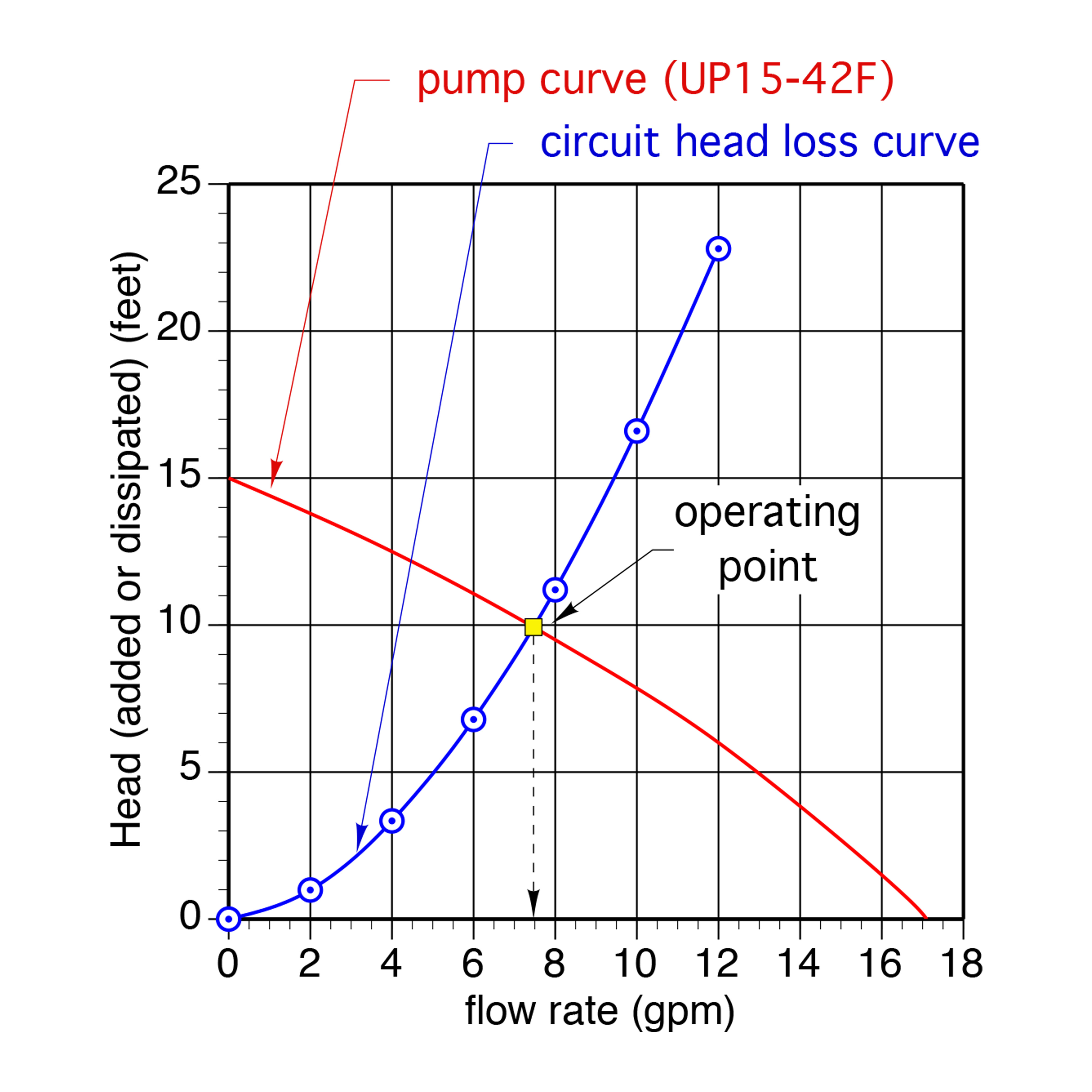
Example: Determine the flow rate for the circuit shown in Figure 5-14, assuming a UP15-42F circulator is used (pump curve shown in Figure 5-21). The circuit operates with an average water temperature of 140ºF.
Solution: The system curve for this piping system operating with the stated conditions has already been determined and is shown in Figure 5-18. If this curve is plotted on the same graph with the pump curve of the UP15-42F circulator, the operating point is easily determined as shown in Figure 5-24.
Drawing a line from the operating point to the horizontal axis indicates that the circuit will operate at a flow rate of about 7.5 gpm.
HYDRAULIC SEPARATION
Many hydronic systems contain multiple independently controlled circulators. These circulators can vary significantly in their flow and head characteristics. Some may operate at constant speed, while others will operate at variable speeds.
When two or more circulators operate simultaneously in the same system, they each attempt to establish differential pressures based on their own pump curves.
Ideally, each circulator in a system should establish a differential pressure and flow rates that is unaffected by the presence of another operating circulator within the system. When this desirable condition is established, the circulators are said to be hydraulically separated from each other.
Conversely, the lack of hydraulic separation can create very undesirable operating conditions in which circulators interfere with each other. The resulting flows and rates of heat transport within the system can be greatly affected by such interference, often to the detriment of proper heat delivery.
The degree to which two or more operating circulators interact with each other depends on the head loss of the piping path they have in common. This piping path is called the “common piping,” since it is in common with both circuits. The lower the head loss of the common piping, the less the circulators will interfere with each other. Figure 5-25 illustrates this principle for a system with two independently operated circuits.
In this system, both circuits share common piping. The spacious geometry of this common piping creates very low flow velocity through it. As a result, very little head loss or pressure drop can occur across it.


Assume that circulator 1 is operating, but that circulator 2 is off. The lower (blue) system head loss curve in Figure 5-26 applies to this situation.
The point where this lower system head loss curve crosses the circulator’s pump curve establishes the flow rate in circuit 1.
Next, assume circulator 2 is turned on and circulator 1 remains on. The flow rate through the common piping increases, and so does the head loss and pressure drop across it. However, because of its spacious geometry, the increase in head loss and pressure drop is very slight. The system head loss curve that is now seen by circulator 1 has very slightly steepened. It is the upper (green) curve shown in Figure 5-26. The operating point of circuit 1 has moved very slightly to the left, and as a result, the flow rate through circuit 1 has decreased very slightly.
Such a small change in the flow rate through circuit 1 will have virtually no effect on its ability to deliver heat. Thus, the interference created when circulator 2 was turned on is of no consequence. We could say that this situation represents almost perfect hydraulic separation between the two circulators. One could imagine a hypothetical situation in which the head loss across the common piping was zero, even with both circuits operating. Because no head loss occurs across the common piping, it would be impossible for either circulator to have any effect on the other circulator.
Such a condition would represent “perfect” hydraulic separation and would be ideal. Fortunately, perfect hydraulic separation is not required to ensure that the flow rates through independently operated circuits, each with their own circulator and each sharing the same low head loss common piping, remain reasonably stable, and thus are capable of delivering consistent heat transfer.

With good hydraulic separation, the simultaneously operating circulators can barely detect each other’s presence within the system. Thus, each circuit operates as if it were an independent circuit. One can think of circuits that are hydraulically separated as if they were physically disconnected from each other, as illustrated in Figure 5-27.
Any component or combination of components that has very low head loss and is common to two or more hydronic circuits can provide hydraulic separation between those circuits.
One way to create low head loss is to keep the flow path through the common piping very short. Another way to create low head loss is to slow the flow velocity through the common piping.
Examples of devices that use these principles include:
• Closely spaced tees
• A tank (which might also serves other purposes in the system)
• A hydraulic separator

The common piping in Figure 5-28 consists of the closely spaced tees and generously sized headers. Because they are positioned as close to each other as possible, there is virtually no head loss between the tees. These tees form the common piping between the heat source circuit and the distribution circuits, and thus provide hydraulic separation between these circuits.
The generously sized headers create low flow velocity and low head loss, and thus provide hydraulic separation between the three distribution circulators. These headers should be sized so that the maximum flow velocity when all circulators served by the header are on is no more than 2 feet per second. Together, these details create hydraulic separation between all four circulators in the system.
The closely spaced tees allow the heat source circulator to only “see” the flow resistance of the heat source and piping between the boiler and closely spaced tees. The heat source circulator doesn’t help move water through the distribution circuits. Likewise, the three distribution circulators are only responsible for circulation through their respective circuits and do not assist in moving flow through the heat source.
Notice also that constant speed and variable-speed circulators, perhaps of different sizes, can be combined onto the same generously sized header system. Interaction between these circulators will be very minimal because of the very low head loss of those headers.

Figure 5-29 shows a buffer tank combined with generously sized headers serving as the low head loss common piping that provides hydraulic separation between the heat source circulator and each of the distribution circulators. This demonstrates that hydraulic separation can sometimes be accomplished as an ancillary function to the main purpose of the device (e.g., hydraulic separation is not the main function of the buffer tank).
Still another method of providing hydraulic separation is through use of a device that is appropriately called a “hydraulic separator.” Figure 5-30 shows a hydraulic separator installed in place of the buffer tank of Figure 5-29. Note the similarity of the piping connections between the buffer tank and hydraulic separator.
Hydraulic separators, which are sometimes also called low loss headers, create a zone of low flow velocity within their vertical body. The diameter of the body is typically three times the diameter of the connected piping. This causes the vertical flow velocity in the vertical body to be approximately 1/9th that of the connecting piping. Such low velocity creates very little head loss and very little pressure drop between the upper and lower connections. Thus, a hydraulic separator provides hydraulic separation in a manner similar to a buffer tank, only smaller.

The reduced flow velocity within a hydraulic separator allows it to perform two additional functions. First, air bubbles can rise upward within the vertical body and be captured in the upper chamber. When sufficient air collects at the top of the unit, the float-type air vent allows it to be ejected from the system. Thus, a hydraulic separator can replace the need for a high-performance air separator.
Second, the reduced flow velocity allows dirt particles to drop into a collection chamber at the bottom of the vertical body. A valve at the bottom can be periodically opened to flush out the accumulated dirt. Thus, the hydraulic separator also serves as a dirt separator.
The ability of modern hydraulic separators to provide three functions—hydraulic separation, air removal and dirt removal—makes them well-suited for a variety of systems, especially systems in which an older distribution system, one that may have some accumulated sludge, is connected to a new heat source.
For a more in-depth discussion on Hydraulic Separation: